How to randomize data given in a list in MS Excel? (Step by Step Guide of proven methods)

Let's assume you have a list of names in two columns, where column A consists of the first names and column B consists of the last names and you want to randomly arrange those names and want that first name and last name of every person always comes together.

[METHOD 1]

Here we are going to randomly arrange data given in a list in MS Excel using RAND function

Step 1: Go to a blank column right next to your data and enter the RAND formula =RAND(), this will give you a random value in the cell.

In Our example we will go to column C and enter the RAND formula right next to the names

Step 2: Now fill down the formula to all the remaining cells by double clicking the fill handle

Step 3: Now select the first cell and Go to >> Home Tab >> Editing group >> Sort and filter >> Sort Largest to Smallest

↓↓
↓↓

This will randomly arrange your names and you can see that first name and last name of a every person is coming together✅

and you can now directly select and delete the data in column C we used to create random numbers, this will not affect your data.

[METHOD 2]

If you want to randomize your data seamlessly using VBA code, then click here

This method will place your newly created randomized data into a new sheet.

[METHOD 3]

Here we are going to randomly arrange data given in a list in MS Excel using RANDBETWEEN function

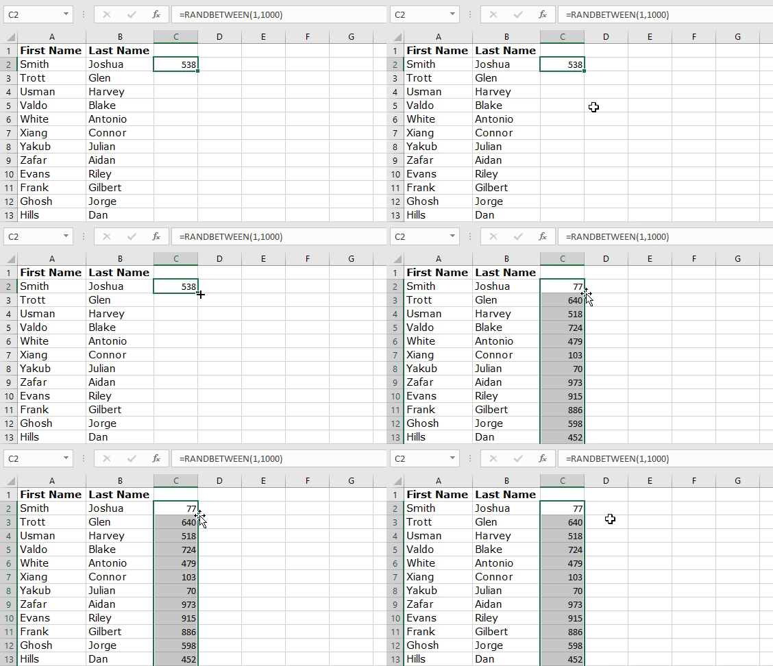
Step 1: Go to a blank column right next to your data and enter the RANDBETWEEN formula =RANDBETWEEN(1,1000), this will give you a random value in the cell ranging from 1 to 1000.

In Our example we will go to column C and enter the RANDBETWEEN formula right next to the names

Step 2: Now fill down the formula to all the remaining cells by double clicking the fill handle

Step 3: Now select the first cell and Go to >> Home Tab >> Editing group >> Sort and filter >> Sort Largest to Smallest

↓↓
↓↓

This will randomly arrange your names and you can see that first name and last name of a every person is coming together✅

and you can now directly select and delete the data in column C we used to create random numbers, this will not affect your data.

If you still have any doubts, you can comment it down below.